


[Editors Note: This is a guest post from Christian Hamson. Christian is the Chief Credit Officer at NSR Invest. He has 20 years experience underwriting and building predictive models specificly for unsecured consumer installment loans. He is now using his expertise to guide the NSRInvest Fund and managed accounts.]
An important and seemingly simple question is how many loans should an investor buy to lower the variance on their expected return to a tolerable level. Part one addressed this issue using the information readily available from Lending Club and Prosper. Several blogs and other posts have also addressed this question.
A few examples of blog posts that have addressed diversification:
- Lending Robot calculates this number to be 146, using Lending Club historical data and a Monte Carlo methodology.
- Peter Renton at Lend Academy calculated a number of ~500 using Prosper data.
- Simon from LendingMemo says at least 200 is best.
What I hope to do in this post is to use traditional statistical methods to estimate the number of loans necessary for adequate diversification.
All of these posts used historical data, differing, but reasonable methodologies, and a few basic assumptions. The Lending Robot post does a great job of making the assumptions they use to calculate an explicit answer. Two key assumptions made in the Lending Robot methodology are:
- The returns on the loans follow a normal distribution. This is a good assumption. The distribution of a proportion is binomial, and for even small sample sizes the normal distribution can be proven to approximate the binomial distribution. The binomial distribution results when there are a number of events (defaults), in n independent experiments (loans), where there are only two possible outcomes (default, or non-default), and an individual default occurs with probability p.
- Any two loans are independent. If one borrower defaults that isn’t likely to change the probability of default of some other borrower.
Assumption: Loan Defaults are not correlated
If I make the same two assumptions as Lending Robot, it is straightforward to calculate the sample size (number of loans an investor ought to buy) using any of the hundreds of sample size calculators freely available on the web. I did a search using Google; and found this tool. I used a margin of error of 5%, a confidence level of 95%, population of 100,000 and a sample proportion of 9.5% (A loss rate that would drive the returns of an investor negative.) With these inputs a sample size of 132 is suggested.
This number is right in the ball park of the Lending Robot, Lending Club, and Prosper, suggestions. Play with the sample size calculators. Put in your own assumptions. Explore. What if loan defaults are not independent? What if borrowers are subject to factors in the economic environment such as unemployment, that cause the probabilities of default to correlate? What should the number of loans for adequate diversification be in this case?
Assumption: Loan Defaults are Correlated to Some Extent
I will repeat the analysis under the assumption that defaults are correlated. Warning! The math gets much, much harder. Suppose default rate is correlated with unemployment rate. Unemployment rates will impact multiple borrowers and thus the probability of default for loans will correlate. Let’s start with some evidence that loan defaults are correlated.
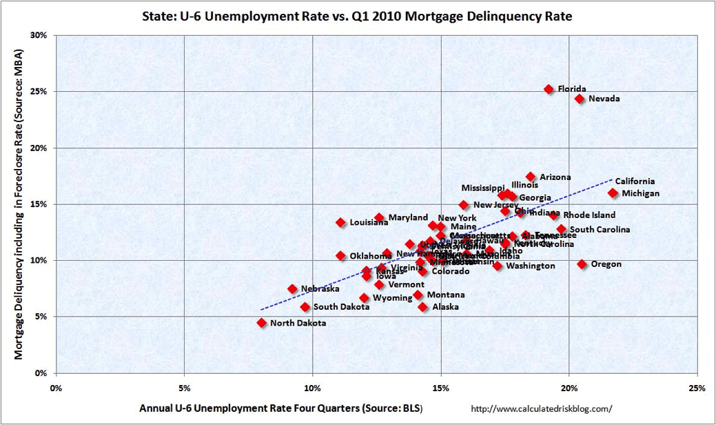
The last recession was a fantastic learning experience. We have a treasure-trove of data (acquired at tremendous expense!) that demonstrates correlation between loan defaults. The above graph is from Calculated Risk. The correlation is obvious to the naked eye. Unsecured installment loans aren’t mortgages, and there were numerous contributors to the mortgage default debacle in addition to unemployment, but at least we have an estimate of the correlation.
The line fit to the data above has an r-square of 0.46, and consequently the correlation between unemployment and mortgage default is 0.68 (The square root of the r-square.) That’s a lot of correlation.
My estimation process of the number of loans needed is based on work done in the medical research field for repeated measures. Suppose we count the number of red blood cells in a patient with anemia, then we give that patient our experimental drug that is supposed to stimulate blood cell production. After a week we count the red blood cells again. Those two counts may differ, but they are obviously correlated.
If we specify a generalized linear model for this case, and input our assumptions for a default rate and correlation, we can, in essence, run the model “backwards” and a number that is usually an input, the number of observations, can be produced as an output. (Note that the repeated measures model is not correct for the loan default situation. A better model would be a hierarchical model.) Since our estimate of correlation is just that, an estimate, we’ll try several values for correlation and determine the dependency of number of loans on correlation. Input values from 0.1 to 0.9 with increments of 0.1.
And the answer is…
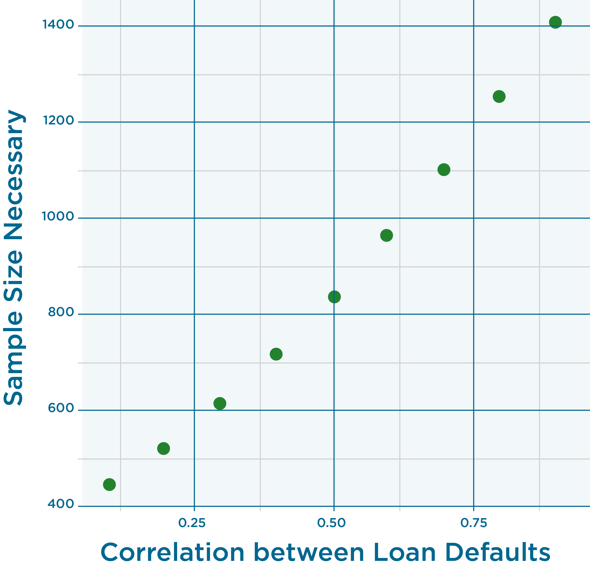
For our estimated correlation of 0.68 at the upper 90% Confidence level the number of loans is 1,070.
Please note that we are using data from the great recession to estimate the correlation rate. In no way, shape or form will 1,070 loans get you through the next recession. That’s a topic for another day, and will not be resolved simply by purchasing more loans. I’d love your thoughts and feedback on this post and methodology. I’d really appreciate someone specifying the hierarchical model and running this analysis again. 🙂